
Introduction
1.1 What is Linear Regression?
Linear regression is a powerful mathematical tool used in machine learning to understand and predict relationships between variables. It is a supervised learning algorithm that aims to find the best-fit line that represents the linear relationship between input variables and a target variable. In simple terms, linear regression helps us draw a straight line through a scatter plot of data points to understand how one variable affects another.
Now, let's dive into a fun story to help us understand linear regression better!
Imagine you are a detective solving a mystery. You have a bag full of colorful balloons, and you want to figure out how the size of the balloons is related to their flying height. Linear regression is like using your detective skills to find clues and solve this exciting mystery.
You start by plotting all the balloons on a graph. The x-axis represents the size of the balloons, and the y-axis represents their flying height. Now, your job is to draw a line that best represents the connection between the size of the balloons and their flying height. This line will help you predict how high a balloon will fly based on its size.
1.2 Applications of Linear Regression
Linear regression has many practical applications in our daily lives. Let's explore some exciting examples:
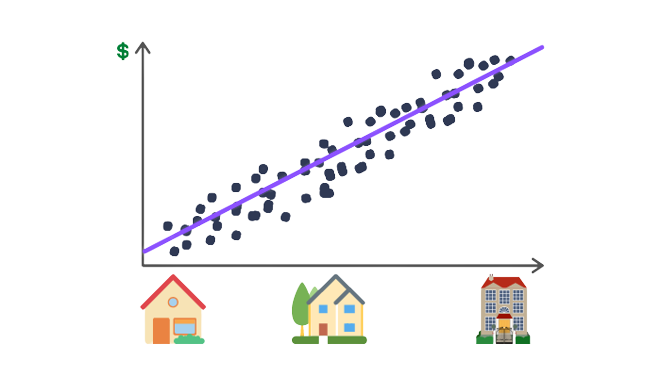
- Predicting House Prices: Imagine you are in the market for a new house. Linear regression can help predict the price of a house based on factors like the number of bedrooms, the size of the house, and its location. This information can guide you in making informed decisions about buying a home.
- Weather Forecasting: Linear regression can be used to predict weather conditions based on historical data. By analyzing factors like temperature, humidity, and air pressure, meteorologists can make accurate predictions about future weather patterns.
- Sports Performance Analysis: Coaches and athletes can use linear regression to analyze data from sports competitions. By examining variables like training time, nutrition, and sleep patterns, they can predict an athlete's performance and make adjustments to improve their results.
1.3 Importance of Linear Regression in Machine Learning
Linear regression is a fundamental technique in machine learning. Here's why it's so important:
- Prediction: Linear regression allows us to make predictions about future outcomes based on historical data. By understanding the relationship between variables, we can estimate values and anticipate results.
- Interpretability: Linear regression provides interpretable results. The coefficients of the line can give us insights into the strength and direction of the relationship between variables. This makes it easier for us to understand and explain the findings.
- Model Building: Linear regression serves as a stepping stone for more complex machine learning algorithms. It helps us build a strong foundation by understanding the basic principles of modeling and prediction.
- Feature Importance: Linear regression can identify the most influential variables in a dataset. By analyzing the coefficients, we can determine which features have the greatest impact on the target variable.
So, linear regression is like being a detective, solving mysteries and making predictions based on the clues hidden in data. By drawing the best-fit line, we can uncover relationships between variables and make informed decisions. Whether it's predicting house prices, analyzing sports performance, or understanding weather patterns, linear regression is a valuable tool in the exciting world of machine learning!
Understanding Linear Regression
2.1 Assumptions of Linear Regression
Linear regression relies on certain assumptions to provide accurate results. These assumptions help us understand the limitations and requirements of the model. Let's explore these assumptions:
- Linearity: The relationship between the input variables and the target variable is assumed to be linear. This means that the relationship can be represented by a straight line on a graph.
- Independence: The observations in the dataset are assumed to be independent of each other. This means that one observation does not influence another.
- Homoscedasticity: The variance of the errors (the differences between the predicted and actual values) should be constant across all levels of the input variables. In simpler terms, the spread of the data points around the best-fit line should be roughly the same across the entire range of the input variables.
- Normality: The errors should follow a normal distribution. This means that the majority of the errors are small, and the extreme errors are rare.
Understanding these assumptions is important because violating them can lead to unreliable results. It's like following a recipe to bake a delicious cake. If we miss an ingredient or deviate from the instructions, the cake may not turn out as expected.
2.2 Simple Linear Regression vs. Multiple Linear Regression
In linear regression, we can distinguish between two types: simple linear regression and multiple linear regression.
Simple Linear Regression: This type of regression involves only one input variable, also known as a predictor variable, to predict the target variable. It's like trying to predict how fast a car will go based on its engine size. We use a straight line to represent the relationship between the input variable and the target variable.
Multiple Linear Regression: In this case, we have multiple input variables that contribute to predicting the target variable. Imagine trying to predict a student's exam score based on variables like study time, sleep duration, and number of extracurricular activities. We use a multi-dimensional space and a plane to represent the relationship between the input variables and the target variable.
2.3 Linear Relationship and Linearity Assumption
Linear regression assumes a linear relationship between the input variables and the target variable. But what does "linear" mean in this context?
Think of a roller coaster ride! In a linear relationship, the changes in the input variables result in proportional changes in the target variable. It's like going up and down on a roller coaster track, where every hill and dip is connected by a straight line.
However, it's important to note that not all relationships are linear. Sometimes, the relationship might be more like a curvy roller coaster ride, with loops and twists. In those cases, linear regression may not be the most suitable approach.
2.4 Best-Fit Line and Residuals
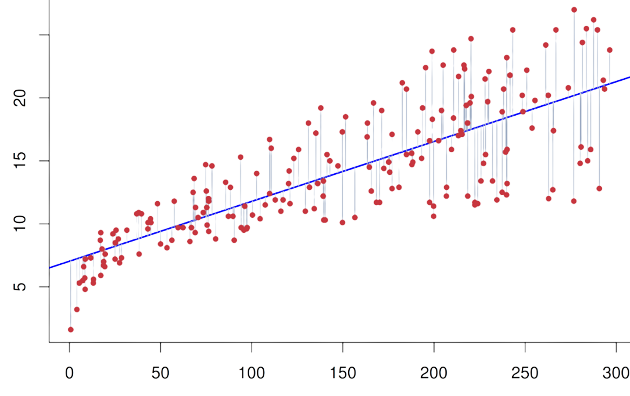
When we plot the data points on a graph, we can draw a line that represents the relationship between the input variables and the target variable. This line is called the "best-fit line" or the "regression line." It's like drawing the smoothest path through the roller coaster track that comes closest to all the data points.
But what happens when the data points don't fall perfectly on the best-fit line? We calculate the differences between the predicted values and the actual values, known as "residuals." These residuals represent the errors in our predictions.
Imagine trying to hit a target with a bow and arrow. If our aim is perfect, the arrow hits the bullseye, and the residual is zero. However, if we miss the bullseye, the arrow lands either above or below the target, and the residual represents the distance of the miss.
In linear regression, our goal is to minimize these residuals, making the best-fit line as accurate as possible. It's like sharpening our archery skills to hit the bullseye consistently.
By understanding these concepts of assumptions, types of regression, linearity, and residuals, we gain valuable insights into the world of linear regression. It's like unraveling the secrets of a roller coaster ride and practicing our archery skills to improve our aim. Linear regression empowers us to understand relationships between variables and make predictions that can help solve real-world problems!
Building a Linear Regression Model
3.1 Dataset and Variables
To build a linear regression model, we need a dataset consisting of observations or examples. Each observation contains information about the input variables (also known as independent variables or features) and the target variable (also known as the dependent variable or outcome variable).
Let's imagine we are trying to predict a person's height based on their age and weight. The dataset would contain different people's information, such as their age, weight, and height. Each person's data is like a puzzle piece that helps us understand the relationship between age, weight, and height.
3.2 Estimating Coefficients
Coefficients play a crucial role in linear regression. They represent the values that determine the relationship between the input variables and the target variable. Estimating these coefficients means finding the best values that fit the data and help make accurate predictions.
Continuing with our example, we want to estimate the coefficients that define how age and weight contribute to a person's height. It's like finding the right puzzle pieces that fit together to create a complete picture. The coefficients act as the puzzle pieces that connect the input variables to the target variable.
3.3 Intercept and Slope of the Line
In linear regression, the intercept and slope of the line are essential components of the model. They determine the position and steepness of the line, respectively.
The intercept is like the starting point of a roller coaster ride. It represents the height at which the ride begins. In our example, the intercept represents the predicted height when age and weight are both zero. It's like the height of a person who is newborn and has no weight.
The slope of the line indicates how much the target variable changes when the input variable changes. Imagine going up a roller coaster hill. The steeper the hill, the faster you climb. Similarly, the slope of the line in our example tells us how much a person's height increases for every unit increase in age or weight.
3.4 Model Representation
Once we have estimated the coefficients, intercept, and slope, we can represent the linear regression model mathematically. It's like writing down the instructions for building a roller coaster or solving a puzzle.
In our example, the model representation would be a mathematical equation that expresses the predicted height as a function of age and weight. It might look like this: Height = Intercept + (Coefficient_Age × Age) + (Coefficient_Weight × Weight). This equation allows us to plug in different values for age and weight and predict the corresponding height.
Cost Function and Gradient Descent
4.1 Introduction to the Cost Function:
The cost function, also known as the mean squared error (MSE), is a mathematical formula that measures how well our linear regression model fits the data. It calculates the difference between the predicted values and the actual values.
Imagine you are playing a dart game, and you want to hit the bullseye. The cost function tells you how far off your dart hits are from the center of the target. The closer your darts land to the bullseye, the lower the cost.
The formula for the cost function in linear regression is:
cost = (1/2m) * Σ(yᵢ - ŷᵢ)²
In this formula, m represents the number of data points, yᵢ is the actual value of the target variable for each data point, and ŷᵢ is the predicted value by the linear regression model.
4.2 Minimizing the Cost Function:
The goal of linear regression is to find the coefficients and intercept that minimize the cost function. We want to adjust these values so that our predictions are as close as possible to the actual values.
Imagine you are on a treasure hunt, and you have a metal detector. You move around, adjusting the settings on the detector to find the buried treasure. The cost function is like a guide that tells you how close you are to the treasure. Your goal is to minimize the cost, which means getting closer to the treasure.
To minimize the cost function, we use an optimization algorithm called gradient descent.
4.3 Gradient Descent Algorithm:
The gradient descent algorithm helps us minimize the cost function by iteratively updating the coefficients and intercept. It guides us in the right direction, like a treasure map leading us to the buried treasure.
Imagine you are on a mountain and you want to reach the bottom. You take steps in the direction of steepest descent to get to the lowest point. The gradient descent algorithm tells you which way to go and how big of a step to take.
The update rule for gradient descent in linear regression is:
θⱼ = θⱼ - α * (∂J/∂θⱼ)
In this formula, θⱼ represents the jth coefficient, α is the learning rate, J is the cost function, and (∂J/∂θⱼ) is the partial derivative of the cost function with respect to θⱼ.
By updating the coefficients and intercept based on the gradient descent algorithm, we gradually improve our linear regression model's fit to the data.
4.4 Learning Rate and Convergence:
The learning rate is a parameter that determines the size of the steps we take during each iteration of gradient descent. It's like the pace at which we move towards the minimum cost.
Imagine you are exploring a maze, and you have control over how big of a step you take. A small step allows you to carefully navigate the maze, while a large step might lead you to skip important turns.
Finding the right learning rate is crucial. If the learning rate is too small, it may take a long time to reach the minimum cost. On the other hand, if the learning rate is too large, you may overshoot the minimum and fail to converge.
Convergence refers to the point where our model has reached the minimum cost and has stabilized. It's like finally reaching the bottom of the mountain and stopping. We want our model to converge quickly and accurately so that we can make accurate predictions.
By understanding the concepts of the cost function, minimizing it through gradient descent, the gradient descent algorithm, learning rate, and convergence, we can fine-tune our linear regression model and aim for the bullseye with our dart. It's like becoming a skilled treasure hunter who can navigate the terrain and make smart decisions to find the buried treasure!
Model Evaluation Metrics
5.1 Mean Squared Error (MSE):
The Mean Squared Error (MSE) is a metric used to measure the average squared difference between the predicted values and the actual values in a linear regression model. It gives us an idea of how well our model is performing in terms of prediction accuracy.
Imagine you are a chef, and you want to know how accurately you can estimate the weight of ingredients in a recipe. The MSE would be like measuring the squared difference between your estimated weights and the actual weights of the ingredients. The lower the MSE, the more accurate your estimations.
The formula for MSE is:
MSE = (1/m) * Σ(yᵢ - ŷᵢ)²
Here, m represents the number of data points, yᵢ is the actual value of the target variable for each data point, and ŷᵢ is the predicted value by the linear regression model.
5.2 Root Mean Squared Error (RMSE):
The Root Mean Squared Error (RMSE) is similar to MSE but provides a more interpretable metric by taking the square root of the MSE. It gives us a sense of the average difference between the predicted values and the actual values, in the same units as the target variable.
Let's go back to the chef example. If you want to understand how far off your weight estimations are from the actual weights of the ingredients, the RMSE would give you an idea of the average difference in weight, like the average distance between your estimations and the actual weights.
The formula for RMSE is:
RMSE = √(MSE)
5.3 Coefficient of Determination (R-squared):
The Coefficient of Determination, commonly known as R-squared, is a metric that represents the proportion of variance in the target variable that is explained by the linear regression model. It measures how well the model fits the data.
Think of a student taking a test. The R-squared value would indicate how much of the student's performance on the test can be attributed to their studying and preparation. The higher the R-squared value, the more the model can explain and predict the target variable.
The R-squared value ranges from 0 to 1, where 0 indicates that the model explains none of the variance and 1 indicates that the model explains all the variance in the target variable.
5.4 Interpreting Evaluation Metrics:
When evaluating a linear regression model, we look at the MSE, RMSE, and R-squared to understand its performance.
- MSE and RMSE: We want these metrics to be as low as possible. A lower MSE or RMSE indicates that the model's predictions are closer to the actual values. It shows that the model is making more accurate predictions.
- R-squared: We want this metric to be as close to 1 as possible. A higher R-squared value suggests that the model is capturing a larger proportion of the variance in the target variable, indicating a better fit to the data.
By analyzing these evaluation metrics, we can assess the performance of our linear regression model and make informed decisions about its effectiveness in predicting the target variable.
Summary
6.1 Key Concepts of Linear Regression:
In linear regression, we use mathematical techniques to find the best-fit line that predicts the relationship between input variables and a target variable. The key concepts of linear regression include assumptions, building a regression model, cost function and gradient descent, and model evaluation metrics.
6.2 Practical Applications and Limitations:
Linear regression has numerous practical applications. It can be used to predict housing prices based on factors like the number of bedrooms, area, and location. It is also used in finance to predict stock prices or analyze the impact of interest rates on investments. However, linear regression has limitations. It assumes a linear relationship between variables, and if the relationship is nonlinear, the model may not perform well.
6.3 Importance of Model Evaluation:
Model evaluation is essential to assess the performance and accuracy of our linear regression model. Evaluation metrics like MSE, RMSE, and R-squared help us understand how well our model fits the data and makes predictions. It allows us to compare different models and make improvements if needed.
For example, imagine you are a coach of a basketball team. To evaluate your team's performance, you track their shooting accuracy and the number of points scored. Similarly, in linear regression, model evaluation helps us understand how well our model performs and guides us in making necessary adjustments.
6.4 Next Steps in Machine Learning Journey:
After learning about linear regression, there are several exciting paths to explore in the machine learning journey. You can delve into other regression techniques like polynomial regression, or explore classification algorithms like logistic regression. Additionally, you can dive into more advanced machine learning algorithms such as decision trees, support vector machines, or neural networks.