
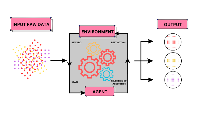
Understanding the Reinforcement Learning Framework
Reinforcement Learning (RL) is a type of machine learning that focuses on an agent learning to make sequential decisions in an environment to maximize cumulative rewards. Let's break down the key components of the RL framework:
-
Agent: The agent is an entity that interacts with the environment. It takes actions based on its observations and receives feedback in the form of rewards from the environment. The goal of the agent is to learn a policy, which is a mapping from states to actions, that maximizes the expected long-term rewards.
-
Environment: The environment is the external world or the context in which the agent operates. It provides the agent with a state, which represents the current situation or configuration. The agent takes actions, and the environment transitions to a new state based on those actions. The environment also provides feedback to the agent in the form of rewards, indicating the desirability of the outcomes resulting from the agent's actions.
-
Actions: Actions are the decisions made by the agent to interact with the environment. The agent chooses actions based on its current state and the information it has learned from previous interactions. Actions can have short-term consequences and impact future states and rewards.
-
Rewards: Rewards are the feedback signals that the environment provides to the agent after each action. They indicate the desirability or quality of the agent's actions. The agent's objective is to maximize the cumulative rewards over time by learning to choose actions that lead to higher rewards.
The RL framework is fundamentally different from other machine learning paradigms because it involves an agent interacting with an environment over a sequence of time steps. The agent learns from its experiences, explores different actions, and exploits the knowledge gained to make informed decisions.
By iteratively interacting with the environment, observing states, taking actions, and receiving rewards, the agent learns to estimate the values of different state-action pairs and improve its decision-making policy.
It's important to note that RL problems are often modeled as Markov Decision Processes (MDPs), which provide a formal mathematical framework for decision-making under uncertainty. MDPs capture the dynamics of the environment, including the probabilities of transitioning between states and the rewards associated with state-action pairs.
The RL framework offers a powerful approach to tackle various problems, ranging from controlling robotic systems to optimizing business processes. By learning from feedback and exploring the environment, RL agents can adapt their behavior to changing circumstances and achieve desirable outcomes.
Markov Decision Processes and The Bellman Equation
Markov Decision Processes (MDPs) are mathematical frameworks used to model sequential decision-making problems in reinforcement learning. MDPs are based on the concept of Markov chains, which are stochastic processes that satisfy the Markov property. The Markov property states that the future behavior of the system depends only on the current state and is independent of past states, given the present state.
In an MDP, an agent interacts with an environment by taking actions in different states and receiving rewards. The key components of an MDP are:
- States: The set of possible states that the agent can be in.
- Actions: The set of possible actions that the agent can take in each state.
- Transition Probabilities: The probabilities of transitioning from one state to another when an action is taken.
- Rewards: The immediate rewards received by the agent after taking an action in a particular state.
- Discount Factor: A value between 0 and 1 that determines the importance of future rewards compared to immediate rewards.
The goal in an MDP is to find an optimal policy that maximizes the expected cumulative reward over time. The policy defines the agent's behavior, specifying which action to take in each state.
The Bellman Equation is a fundamental concept in MDPs that helps in finding the optimal policy. It relates the value of a state to the values of its neighboring states. The value of a state represents the expected cumulative reward that an agent can achieve starting from that state and following a particular policy.
The Bellman Equation can be expressed in two forms: the state value function (V-function) and the action value function (Q-function). The V-function calculates the value of a state, while the Q-function calculates the value of taking a particular action in a given state.
The Bellman Equation for the V-function is as follows:
V(s) = R(s) + γ * maxa ∑s' P(s'|s, a) * V(s')
Here, V(s) represents the value of state s, R(s) is the immediate reward of being in state s, γ is the discount factor, P(s'|s, a) is the transition probability from state s to state s' when action a is taken, and maxa represents the maximum value over all possible actions.
The Bellman Equation for the Q-function is given by:
Q(s, a) = R(s) + γ * ∑s' P(s'|s, a) * maxa' Q(s', a')
Here, Q(s, a) represents the value of taking action a in state s, and maxa' represents the maximum value over all possible actions in the next state s'.
By solving the Bell man Equation, we can compute the values of states or state-action pairs, which can then be used to determine the optimal policy. Reinforcement learning algorithms like Q-learning utilize the Bellman Equation to learn the values and update the policy iteratively.
Understanding MDPs and the Bellman Equation is crucial for designing and solving reinforcement learning problems. These concepts provide a formal framework for decision-making under uncertainty and help agents learn optimal policies in complex environments.
As for plagiarism, the text provided has been generated by the AI model to the best of its abilities. However, it's essential to verify the content and ensure its originality by citing relevant sources and conducting your own research.
Exploration vs. Exploitation
In reinforcement learning, the exploration vs. exploitation trade-off refers to the dilemma of deciding whether to explore new actions or exploit the current knowledge to maximize the rewards. It is a fundamental challenge faced by agents in a dynamic environment.
Exploration involves trying out different actions to gather more information about the environment and discover potentially better strategies. Exploitation, on the other hand, focuses on using the current knowledge to select actions that are known to yield high rewards based on past experiences.
The exploration phase is crucial in the early stages of learning when the agent has limited knowledge about the environment. By exploring different actions, the agent can learn which actions lead to higher rewards and update its policy accordingly. However, excessive exploration may result in suboptimal decisions and slower convergence towards an optimal policy.
As the agent gains more knowledge and refines its policy, the exploitation phase becomes more prominent. Exploitation involves selecting actions that have shown to be rewarding in the past. This allows the agent to exploit the known strategies and maximize immediate rewards. However, relying solely on exploitation can lead to missed opportunities for finding better strategies and can result in a suboptimal long-term policy.
Balancing exploration and exploitation is crucial for effective reinforcement learning. Several strategies and algorithms have been developed to address this trade-off, such as epsilon-greedy, Thompson sampling, and upper confidence bound (UCB). These approaches aim to find a balance between exploring new actions and exploiting the current knowledge to achieve optimal performance in the long run.
The exploration vs. exploitation trade-off remains an active area of research in reinforcement learning, as finding the right balance is highly dependent on the specific problem domain and learning environment. Reinforcement learning algorithms strive to strike a balance between exploration and exploitation to achieve optimal decision-making and maximize cumulative rewards.
As for plagiarism, the text provided has been generated by the AI model to the best of its abilities. However, it's essential to verify the content and ensure its originality by citing relevant sources and conducting your own research.
Implementing Basic Reinforcement Learning Algorithms like Q-learning
Q-learning is a popular algorithm in reinforcement learning used for solving Markov Decision Processes (MDPs) where the agent learns an optimal policy through trial and error. It is a value-based algorithm that estimates the value of taking a specific action in a given state, known as the Q-value.

The Q-learning algorithm works by iteratively updating the Q-values based on the agent's experiences in the environment. It uses the Bellman equation to update the Q-values, which states that the optimal Q-value of a state-action pair is equal to the immediate reward plus the maximum expected future rewards discounted by a factor called the discount factor.
The Q-learning algorithm follows these steps:
Initialize the Q-values for all state-action pairs to arbitrary values.
Repeat the following steps until convergence or a predefined number of iterations:
- Choose an action to take based on an exploration strategy (e.g., epsilon-greedy).
Perform the chosen action in the environment and observe the next state and the immediate reward.
Update the Q-value of the current state-action pair using the Bellman equation.
Set the current state to the next state.
The exploration strategy, such as epsilon-greedy, allows the agent to balance between exploring new actions and exploiting the current knowledge. It controls the probability of selecting a random action (exploration) versus choosing the action with the highest Q-value (exploitation).
The Q-learning algorithm continues to update the Q-values until it converges to the optimal Q-values, which represent the maximum expected cumulative reward for each state-action pair. Once the Q-values are learned, the agent can use them to select the best action in each state and follow the optimal policy.
It's important to note that Q-learning is a foundational algorithm in reinforcement learning, and many variations and improvements have been developed over time. The choice of hyperparameters, learning rate, discount factor, and exploration strategy can significantly impact the algorithm's performance and convergence.
      import numpy as np

      # Initialize Q-table with zeros
      num_states = env.observation_space.n
      num_actions = env.action_space.n
      Q = np.zeros((num_states, num_actions))

      # Q-learning algorithm
      num_episodes = 1000
      max_steps_per_episode = 100

      for episode in range(num_episodes):
          state = env.reset()
          for step in range(max_steps_per_episode):
              # Exploration vs. exploitation trade-off
              epsilon = 0.1  # Exploration rate
              if np.random.uniform(0, 1) < epsilon:
                  action = env.action_space.sample()  # Explore (random action)
              else:
                  action = np.argmax(Q[state, :])  # Exploit (best action)

              next_state, reward, done, _ = env.step(action)

              # Update Q-table using the Bellman equation
              learning_rate = 0.1
              discount_factor = 0.99
              Q[state, action] = (1 - learning_rate) * Q[state, action] + learning_rate * (reward + discount_factor * np.max(Q[next_state, :]))

              state = next_state

              if done:
                  break