Introduction to Neural Networks

Definition of Neural Networks: Neural networks are powerful machine learning models inspired by the structure and functionality of the human brain. They are widely used for various tasks like image classification, natural language processing, and more. In this lesson, we will explore the basic structure of neural networks, the feedforward process, activation functions, and how to implement a basic neural network using TensorFlow or PyTorch.

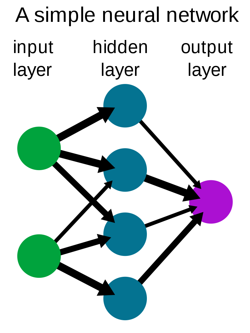
Understanding the basic structure of neural networks: Neural networks are composed of interconnected nodes called neurons. These neurons are organized into layers: an input layer, one or more hidden layers, and an output layer. Each neuron receives input from the previous layer, applies a transformation, and passes the output to the next layer. The strength of these connections is represented by weights, which are learned during the training process.

Understanding the basic structure of neural networks can be related to the structure and functionality of the human brain. Just like the brain consists of interconnected neurons, neural networks are composed of artificial neurons called nodes. In the human brain, neurons are the fundamental building blocks responsible for transmitting and processing information. Similarly, in neural networks, nodes perform similar functions. They receive inputs, apply transformations, and pass the output to the next layer. Let's consider a simple example to illustrate this analogy:

Understanding Neural Networks with Human Brain Analogy

Imagine you want to teach a child to identify different shapes, such as circles and triangles. In the human brain, there are specialized neurons responsible for recognizing shapes. These neurons receive visual information as input and activate when they identify a specific shape.

Now, let's translate this into the context of neural networks. We can represent the visual input as numerical data, where each feature represents a specific aspect of the shape, such as its size or color. These features serve as inputs to the artificial neurons in the neural network.

In the first layer of the neural network, known as the input layer, the numerical features representing the shape are passed to the neurons. Each neuron in the input layer receives a different feature of the shape. For example, one neuron may receive the size information, while another neuron may receive the color information.

As the information flows through the neural network, it reaches the hidden layers. In the brain analogy, we can consider these hidden layers as interconnected regions of the brain responsible for processing and analyzing the shape's features. Each artificial neuron in the hidden layers receives inputs from the previous layer, performs a weighted sum of those inputs, and applies an activation function.

The activation function plays a crucial role in introducing non-linearity to the neural network, allowing it to learn complex patterns. Just like the brain's neurons activate when they recognize a specific shape, the artificial neurons in the neural network activate based on the patterns they detect in the data.

Finally, the processed information flows through the output layer, which represents the final decision or prediction of the neural network. In our shape recognition example, the output layer may contain neurons representing different shapes like circles and triangles. The activation of the neuron associated with a specific shape indicates the network's prediction of that shape.

Understanding the basic structure of neural networks

Neural networks are composed of interconnected nodes called neurons. These neurons are organized into layers: an input layer, one or more hidden layers, and an output layer. Each neuron receives input from the previous layer, applies a transformation, and passes the output to the next layer. The strength of these connections is represented by weights, which are learned during the training process.

The feedforward process is the fundamental operation in a neural network. It involves passing input data through the network to obtain predictions. Let's break down the feedforward process into simpler steps:

1. Input Layer:

   • The feedforward process starts with the input layer of the neural network.
   • The input layer receives the raw input data, which can be in the form of numerical features, images, or any other suitable format.
   • Each neuron in the input layer represents a specific feature or attribute of the input data.

2. Hidden Layers:

   • After the input layer, the data flows through one or more hidden layers.
   • Each hidden layer consists of multiple neurons that perform computations on the input data.
   • Neurons in the hidden layers receive inputs from the previous layer and apply a weighted sum of those inputs.
   • The weighted sum is obtained by multiplying each input with a corresponding weight value.
   • The weighted sum is then passed through an activation function, which introduces non-linearity to the network.
   • The activation function transforms the weighted sum into an output value that is sent to the next layer.

3. Output Layer:

   • Finally, the processed information reaches the output layer of the neural network.
   • The output layer consists of neurons that represent the final predictions or outputs of the network.
   • The neurons in the output layer apply the same process as in the hidden layers: they receive inputs, apply a weighted sum, and pass the result through an activation function.
   • The choice of activation function in the output layer depends on the specific problem being solved.
   • For example, in a binary classification task, the output layer may use the sigmoid activation function to produce a probability value between 0 and 1 for each class.
   • In a multi-class classification task, the output layer may use the softmax activation function to produce a probability distribution over multiple classes.

The output of the feedforward process is the prediction or output value generated by the neural network. This prediction represents the network's interpretation of the input data based on the learned weights and biases. The goal of training a neural network is to adjust these weights and biases through the learning process, such as backpropagation, so that the network can make accurate predictions for new, unseen data.

Activation Function

Activation functions play a crucial role in neural networks by introducing non-linearity to the output of a neuron. They determine whether a neuron should be activated or not based on the weighted sum of its inputs. Activation functions are responsible for adding complexity and enabling neural networks to learn and represent complex patterns in the data.

There are several commonly used activation functions, including the sigmoid function, the rectified linear unit (ReLU), and the softmax function.

1. Sigmoid Function:

   • The sigmoid function takes a real-valued input and squashes it to a value between 0 and 1.
   • It has an S-shaped curve, and its output can be interpreted as a probability or a measure of confidence.
   • In binary classification tasks, the sigmoid function is often used in the output layer to produce the probability of the positive class.
   • However, the sigmoid function can suffer from the vanishing gradient problem, limiting its effectiveness in deep neural networks.

2. ReLU (Rectified Linear Unit):

   • The ReLU function takes the input value and returns it if it is positive, or 0 otherwise.
   • ReLU is computationally efficient and has been found to work well in many deep learning applications.
   • It overcomes the vanishing gradient problem and allows the network to learn faster and achieve better performance.
   • However, ReLU can suffer from the "dying ReLU" problem, where neurons become inactive and output 0 for all inputs.

3. Softmax Function:

   • The softmax function is commonly used in the output layer for multi-class classification tasks.
   • It takes a vector of real numbers as input and converts them into a probability distribution.
   • The output of the softmax function represents the probabilities of each class, and the sum of all probabilities is 1.
   • The class with the highest probability is typically considered the predicted class.

It's important to choose the appropriate activation function based on the specific problem and network architecture. Experimentation and empirical evaluation are often required to determine the most suitable activation function for a given task.

Practical Implementation of Neural Networks

Implementing a basic neural network involves a few key steps. Let's break them down in an easy-to-understand manner:

1. Data Preparation:

   • Begin by preparing your data. This typically involves dividing your dataset into training and testing sets.
   • Make sure your data is properly formatted and preprocessed, such as scaling numerical features or one-hot encoding categorical variables.

2. Building the Neural Network:

   • Select a deep learning framework like TensorFlow or PyTorch to build your neural network. These frameworks provide convenient tools and functions for creating and training models.
   • Define the architecture of your neural network. Specify the number of layers, the number of neurons in each layer, and the activation functions to be used.
   • Initialize the weights and biases of the neural network. Random initialization is commonly used to avoid symmetry issues during training.

3. Forward Propagation:

   • Perform the feedforward process to obtain predictions from your neural network.
   • Pass your input data through the layers of the network, applying the activation functions to the weighted sums of the inputs.
   • The output layer will produce the final predictions based on the learned parameters of the network.
   

4. Loss Calculation:

   • Compute the loss or error between the predicted outputs and the actual labels in your training data.
   • Choose an appropriate loss function depending on the problem type. For example, mean squared error (MSE) is commonly used for regression tasks, while cross-entropy loss is often used for classification problems.

5. Backpropagation and Gradient Descent:

   • Update the weights and biases of the network to minimize the loss and improve the accuracy of the predictions.
   • Perform backpropagation, which calculates the gradients of the loss with respect to the network parameters.
   • Use an optimization algorithm, such as gradient descent, to adjust the weights and biases in the direction that reduces the loss.

6. Training and Evaluation:

   • Train your neural network by repeating the forward propagation, loss calculation, and backpropagation steps on your training data for multiple iterations or epochs.
   • Monitor the performance of your network on a separate validation set during training to avoid overfitting.
   • Evaluate your trained model on the testing set to assess its generalization performance.

7. Fine-tuning and Hyperparameter Optimization:

   • Experiment with different hyperparameters, such as learning rate, batch size, and number of hidden layers, to optimize the performance of your neural network.
   • Fine-tune your model by adjusting the architecture, activation functions, or regularization techniques like dropout or batch normalization.

Remember, implementing a neural network is an iterative process that requires experimentation, tuning, and analyzing the results to improve its performance. Each problem is unique, so it's important to adapt your network architecture and hyperparameters accordingly.

Check out are Deep Learning page, to get to know about different types of DL models and their usage in the most efficient way.