Overview of CNN Architecture

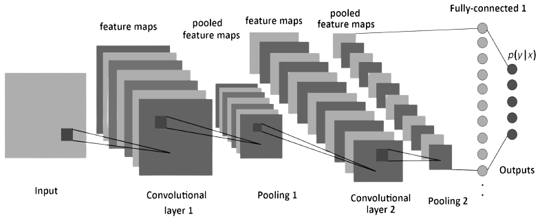
Convolutional Neural Networks (CNNs) are designed specifically for analyzing visual data, such as images. The architecture of a CNN consists of multiple types of layers, each serving a specific purpose.

In simple terms, CNNs use convolutional layers to extract relevant features from input images, pooling layers to reduce spatial dimensions, and fully connected layers to learn complex relationships and make predictions. This architecture allows CNNs to effectively capture patterns and features in visual data.

1. Convolutional Layers:

   • Convolutional layers are the main building blocks of CNNs.

   • These layers apply filters to input images, which helps the network detect local patterns and features.
   • Filters are small matrices that are convolved (slid) across the image to perform element-wise multiplication and summation.
   • Each filter extracts specific features, such as edges or textures, from the input image.
   • The output of a convolutional layer is called a feature map, which represents the presence of different features in the input image.
   • Multiple filters can be applied in parallel to capture different features simultaneously.


2. Pooling Layers:

   • Pooling layers reduce the spatial dimensions of the feature maps.

   • The most common type of pooling is max pooling, where the maximum value within a defined window is selected and retained.
   • Pooling helps to achieve translation invariance by capturing the most important information while reducing the computational complexity.
   • By downsampling the feature maps, pooling layers make the network more robust to variations in the position or scale of the features.

3. Fully Connected Layers:

   • Fully connected layers connect every neuron in one layer to every neuron in the next layer, similar to traditional neural networks.

   • These layers enable the network to learn complex relationships between the features extracted by the convolutional and pooling layers.
   • The fully connected layers are typically placed at the end of the network and are responsible for making the final predictions.

Filters and Feature Maps

1. Filters:

   • Filters are small matrices that are applied to an input image during the convolutional operation.

   • Each filter acts as a feature detector, searching for specific patterns or characteristics within the image.
   • For example, a filter may specialize in detecting edges, corners, or textures.
   • Filters are typically small in size, such as 3x3 or 5x5, and are represented by learnable weights.
   • The values of these weights are adjusted during the training process to optimize the network's performance.
   • By convolving filters across the entire image, CNNs can detect and extract relevant features.

2. Feature Maps:

   • Feature maps are the output of applying filters to the input image.

   • Each filter produces a corresponding feature map, which represents the presence or intensity of a specific feature within the image.
   • The size of a feature map is determined by the dimensions of the input image and the filter.
   • In a grayscale image, a feature map is a 2D matrix where each element represents the activation of a particular filter at a specific location.
   • In a colored image, feature maps are produced for each color channel (e.g., red, green, blue).
   • Multiple filters can be applied in parallel, resulting in a stack of feature maps that capture different features simultaneously.
   • These feature maps serve as inputs for subsequent layers in the CNN architecture.

Here's an example code snippet to illustrate the concept:

    import tensorflow as tf
    from tensorflow.keras import layers
    
    # Define a convolutional layer with 16 filters
    conv_layer = layers.Conv2D(16, kernel_size=(3, 3), activation='relu', input_shape=(height, width, channels))
    
    # Apply the convolutional layer to an input image
    input_image = tf.random.normal((1, height, width, channels))
    feature_maps = conv_layer(input_image)
    
    # Print the shape of the feature maps
    print(feature_maps.shape)
                            

In this code, we define a convolutional layer with 16 filters. We then apply this layer to an input image using the conv_layer object. The resulting feature_maps represent the output feature maps. We can examine the shape of the feature maps to understand the dimensions and the number of feature maps produced.

By using filters and feature maps, CNNs can effectively capture and represent the essential features of an image, enabling them to learn and make accurate predictions on image-related tasks.

Training CNNs for image classification

1. Dataset Preparation: First, we need to gather a labeled dataset of images for training our CNN. This dataset should contain images of different classes, with each image properly labeled with its corresponding class.

2. Data Preprocessing: Before feeding the images into the CNN, we need to preprocess the data. This typically involves resizing the images to a fixed size, normalizing the pixel values, and splitting the dataset into training and testing sets.

3. Model Architecture: We define the architecture of our CNN. This includes specifying the number and types of layers in the network, such as convolutional layers, pooling layers, and fully connected layers. Each layer extracts different features from the images.

4. Model Compilation: After defining the architecture, we compile the model by specifying the optimizer, loss function, and evaluation metrics. The optimizer updates the network's weights during training, the loss function measures the model's performance, and the evaluation metrics provide additional insights into the model's accuracy.

5. Model Training: We train the CNN using the training dataset. During training, the model learns to recognize patterns and features in the images. The training process involves forward propagation, where the input images pass through the network, and backward propagation, where the network adjusts its weights based on the calculated loss. This process is repeated for multiple epochs, gradually improving the model's performance.

6. Model Evaluation: Once the training is complete, we evaluate the model's performance using the testing dataset. This gives us an estimate of how well the model generalizes to unseen data. We calculate metrics such as accuracy, precision, and recall to assess the model's performance.

7. Fine-tuning and Optimization: Depending on the results, we can fine-tune the model by adjusting hyperparameters or modifying the architecture. We can also apply techniques like regularization or data augmentation to improve the model's performance.

It's important to note that training CNNs for image classification can be a computationally intensive task, requiring a substantial amount of training data and computational resources. However, it's a powerful technique for solving complex image recognition tasks.

Important Points:

• Dataset Loading: The CIFAR-10 dataset is used in this example. Make sure to have the dataset downloaded or available in the correct path.

• Dataset Preprocessing: The pixel values of the images are normalized by dividing them by 255.0. This ensures that the pixel values are in the range of [0, 1].

• CNN Architecture: The CNN architecture consists of convolutional layers, pooling layers, and fully connected layers. The specific architecture used in the code can be modified based on the requirements of the task.

• Compilation: The model is compiled with the Adam optimizer, which is a popular choice for training deep learning models. The loss function used is "sparse_categorical_crossentropy" since the labels are provided as integers. The "accuracy" metric is used for evaluation.

• Training: The model is trained using the fit method, with the training images and labels as input. The number of epochs determines how many times the model will iterate over the entire dataset during training.

• Validation: The performance of the model is evaluated using the test dataset. The validation_data argument in the fit method is used to provide the test images and labels for evaluation during training.

• Evaluation: After training, the model's performance is evaluated using the test dataset. The test loss and test accuracy are calculated and printed.

• Model Tuning: The code provided serves as a basic template. Depending on the problem, you may need to adjust the architecture, hyperparameters, or use additional techniques like regularization or data augmentation to improve the model's performance.

Transfer Learning

Transfer learning is a technique in deep learning where a pre-trained model is used as a starting point for a new task or problem. Instead of training a model from scratch, transfer learning allows us to leverage the knowledge and learned features of an existing model that has been trained on a large dataset.

The main idea behind transfer learning is that the features learned by a model on a large and general dataset can be valuable and applicable to a different but related task or dataset. By utilizing a pre-trained model, we can benefit from its ability to extract high-level features and patterns that are useful for various tasks, even if the new dataset is smaller or different from the original training dataset.

In transfer learning, we typically follow these steps:

1. Select a pre-trained model: Choose a pre-trained model that has been trained on a large-scale dataset, such as ImageNet, which contains millions of labeled images. These pre-trained models are often deep convolutional neural networks (CNNs) that have learned to recognize various objects and features.

2. Remove the last layers: Since the pre-trained model was trained on a different task, the last layers are usually task-specific. We remove these layers, which are responsible for the final classification, and retain the earlier layers that capture more general and abstract features.

3. Add new layers: We add new layers to the pre-trained model. These new layers are initialized randomly and will be trained on our specific task. The architecture and number of layers added can be customized based on the complexity of the new task and available resources.

4. Freeze the pre-trained layers: During training, we freeze the weights of the pre-trained layers to prevent them from being updated. This way, we retain the learned features from the pre-trained model and avoid overfitting on the smaller dataset.

5. Train the model: We train the model using the new dataset, which typically has fewer labeled examples compared to the original pre-training dataset. By training only the newly added layers, we can quickly adapt the model to the new task.

By applying transfer learning, we can benefit from the knowledge and representations learned by the pre-trained model, which can significantly improve the performance and convergence speed, especially when the new dataset is limited. Transfer learning is widely used in various computer vision tasks, such as image classification, object detection, and image segmentation.

It is important to note that while transfer learning can be a powerful technique, it might not always guarantee better performance. Learn more about Transfer Learning. The choice of the pre-trained model, similarity between the original and target tasks, and dataset size all play a crucial role in determining the success of transfer learning for a specific problem.